Maximum amount of adapting the time step in case the Newton-Raphson did not converge within nr_maxcount (solver = 0) or gear_nr_maxcount (solver = 1). The default value is 20.
adapt_stepsize_maxcount= 20Path to a file with alpha-decays. This parameter will only be relevant if use_alpha_decay_file is turned on. An example file could look like:
 sb103   7.84058e+10
 sb104   4.29655e+05
 sb105   1.37511e+10
 sb106   1.03780e+17
 te103   8.30806e+02
 ...
Within this file, first the name of the decaying nucleus is given and afterwards the alpha-decay half-life in seconds.
alpha_decay_file = alpha_decays.datFlag to decide if any alpha-decay that is contained in the reaclib_file should get replaced or not. If this parameter is set to 'yes' (default), all reaclib rates will have priority over the additional alpha-decay rates. This parameter will only be relevant if use_alpha_decay_file is turned on. If alpha_decay_ignore_all is turned on, alpha_decay_src_ignore will become irrelevant.
alpha_decay_ignore_all = noFlag to decide if a alpha-decay that is contained in the reaclib_file should get replaced or not. If the source label is given in this parameter here, all rates with this source label will not get replaced. This parameter will only be relevant if use_alpha_decay_file is turned on and alpha_decay_ignore_all is set to no. Per default, experimentally measured rates with the labels wc07, wc12, and wc17 are not replaced.
alpha_decay_src_ignore = wc12;wc17Maximum proton number to include additional alpha-decays. This parameter will only be relevant if use_alpha_decay_file is turned on. The default value is 184.
alpha_decay_zmax = 200Minimum proton number to include additional alpha-decays. This parameter will only be relevant if use_alpha_decay_file is turned on. The default value is 20.
alpha_decay_zmin = 84This file is used to replace \(\beta\)-decays from the Reaclib file. An example of such a file looks like:
   ...
    ca73    1.268195e-03
    0.0030   0.0000   0.0010   0.0000   0.0020   0.9950   0.0000   0.0000   0.0000   0.0000   0.0000
    ...
This file is only read if use_beta_decay_file is enabled. If additionally the information of the average Q-Value and the average neutrino energy of the decay is known, one can add this info behind the half life, e.g.,
   ...
    ca73    1.268195e-03  2.443690e+01  9.034672e+00
    0.0030   0.0000   0.0010   0.0000   0.0020   0.9950   0.0000   0.0000   0.0000   0.0000   0.0000
    ...
where the first number behind the nucleus name is the half-life, the second number the average Q-value, and the third number the average neutrino energy. This Q-value information is only used in case heating_mode is larger than 0.
beta_decay_file = "@WINNET@/data/beta_decays_moeller_mumpower.dat"Colon seperated string with labels of rates that should not get replaced by the beta_decays. Only the source string of the P0n channel of the reaclib is hereby compared. Experimental rates are ignored per default. This parameter is only relevant if use_beta_decay_file is enabled
beta_decay_src_ignore = wc07;wc12;wc17File that contains the fission fragment probabilities of \(\beta\)-delayed fission in case that fissflag is set to 4 and fission_frag_beta_delayed is set to 3.
An example is given by:
    93  220  574
   0 0 0
   019  048  1.96607e-06
   020  048  2.24289e-05
   020  049  1.88041e-05
   020  050  7.65944e-06
   020  051  1.62040e-06
   021  048  1.17847e-05
   021  049  3.62928e-05
   021  050  5.43032e-05
   ...
Here, the first line specifies the fissioning nucleus (atomic number, mass number) and the amount of fission fragments (39). The second line is a dummy line which is not used within WinNet. From the third line onwards, the fission fragments are specified (atomic number, mass number) together with their yield. The third column therefore adds up to one over all fragments. This file is read only when fissflag was set to four. Noe that the following must hold:
\[ \sum Y(Z,A)\cdot A = A_\text{fiss} \]
with the mass number of the fissioning nucleus \( A_\text{fiss}\). Otherwise an error is raised.
bfission_file= "@WINNET@/data/BFISSION"Calculate the average neutron separation energy in every time step. This can be useful to determine the path of the r-process. If this parameter is set to "yes", an additional column will appear in the file mainout.dat, showing the average neutron separation energy.
calc_nsep_energy = noPath to a file that contains the tabulated chemical potential of electron-positron gas taken from the Helmholtz equation of state Timmes & Arnett 1999. These are used in order to calculate the electron captures and \(\beta\)-decays that are given in the weak_rates_file or for the contribution to the entropy in case of heating_mode greater than 0. The file and chem_pot.f90 is a derivative of what is available at Cococubed. The chem_pot_file is read and used in case the parameter use_timmes_mue is set to yes (which is the default) or when nuclear heating is turned on.
chem_pot_file= "@WINNET@/data/chem_table.dat"Boolean parameter that specifies if snapshots should be done only at specific points in time. In this way, the whole composition can be printed ,e.g., after one year. The file will be stored in the directory snaps/. If set to `‘yes’', a file has to be provided with the parameter snapshot_file.
custom_snapshots = yesThis parameter only has an effect in case use_detailed_balance is enabled. The source labels given within this parameter will be ignored by the detailed balance calculation of WinNet, i.e., no rates will be removed or added for any rates given within the provided source labels.
detailed_balance_src_ignore = rath;kd02This parameter only has an effect in case use_detailed_balance is enabled. The source labels given within this parameter will use the Q-value as given in the rate file for the calculation of the inverse rate. This is independent on whether use_detailed_balance_q_reac is enabled or not.
detailed_balance_src_q_reac = rath;kd02This parameter only has an effect in case use_detailed_balance is enabled. The source labels given within this parameter will use the Q-value as given in the isotopes_file (winvn) by the mass excess for the calculation of the inverse rate. This is independent on whether use_detailed_balance_q_reac is enabled or not.
detailed_balance_src_q_winvn = rath;kd02Function of the average electron-neutrino energies in MeV. Only used when neutrino_mode is set to "analytic".
Enue=16.66 Function of the average electron-antineutrino energies in MeV. Only used when neutrino_mode is set to "analytic".
Enuebar=16.66 Function of the average muon-neutrino and tau neutrino energies in MeV. Only used when neutrino_mode is set to "analytic" and nuflag is 4 or 5.
Enux=16.66 Function of the average muon-antineutrino and tau antineutrino energies in MeV. Only used when neutrino_mode is set to "analytic" and nuflag is 4 or 5.
Enuxbar=16.66 Determine how the hydrodynamic quantities should be calculated once the trajectory has ended. Possible values are:
| Value | Expansion | Literature |
|---|---|---|
| 1 (default) | Adiabatic expansion | Korobkin et al. 2012 |
| 2 | Exponential expansion | - |
| 3 | Expansion with const. velocity | - |
| 4 | Expansion with const. velocity | Fujimoto et al. 2008 |
Most expansion types need a velocity. This velocity is calculated with the help of the parameter extrapolation_width. This parameter specifies how many points of the trajectory are used to calculate a residual velocity. This parameter has to be larger than one. For extrapolation_width \(w\) equal two, the velocity is given by:
\[ v=\frac{r_{N-1}-r_{N}}{t_{N-1}-t_{N}}, \]
with the total number of trajectory points \(N\), radius at the last point of the trajectory \(r_N\), and the last trajectory time \(t_N\). For \(w>2\), the velocity is calculated by:
\[ v=\frac{\left( \sum \limits_{i=N-w} ^N r_i \right) \cdot \left( \sum \limits_{i=N-w} ^N t_i \right) -w \cdot \left( \sum \limits_{i=N-w} ^N r_i \cdot t_i \right) } {\left( \sum \limits_{i=N-w} ^N t_i \right) \cdot \left( \sum \limits_{i=N-w} ^N t_i \right) -w \cdot \left( \sum \limits_{i=N-w} ^N t_i^2 \right) } \]
with radius \(r_i\) at trajectory point \(i\), and time \(t_i\).
extrapolation_width=2Final density in g/ccm. Only used when termination_criterion was set to 2.
final_dens= 1e3 Final temperature in GK. Only used when termination_criterion was set to 2.
final_temp= 0.5 Final time in seconds. Only used when termination_criterion was set to 1.
final_time= 1e15 Parameter to change the fission fragment distribution. Possible values are:
| fissflag | Treatment | Necessary other parameters | Reference |
|---|---|---|---|
| 0 | No fission | - | - |
| 1 | Panov | fission_rates_beta_delayed, fission_format_beta_delayed, fission_rates_n_induced, fission_format_n_induced, fission_rates_spontaneous, fission_format_spontaneous | Panov et al. 2001 |
| 2 | Kodama-Takahashi | fission_rates_beta_delayed, fission_format_beta_delayed, fission_rates_n_induced, fission_format_n_induced, fission_rates_spontaneous, fission_format_spontaneous | Kodama & Takahashi 1975 |
| 3 | Mumpower & Kodama-Takahashi | fission_rates_beta_delayed, fission_format_beta_delayed, fission_rates_n_induced, fission_format_n_induced, fission_rates_spontaneous, fission_format_spontaneous, nfission_file | Mumpower et al. 2020, Kodama & Takahashi 1975 |
| 4 | Custom | fission_rates_beta_delayed, fission_format_beta_delayed, fission_rates_n_induced, fission_format_n_induced, fission_rates_spontaneous, fission_format_spontaneous, fission_frag_n_induced, fission_frag_spontaneous, fission_frag_beta_delayed | - |
For fission flag 3, the fragments of Mumpower et al. 2020 are used for beta delayed and neutron induced fission. For spontaneous fission the fragments of Kodama & Takahashi 1975 are used. Also in case of a missing fragment distribution for the rate, the scheme relies on Kodama & Takahashi 1975.
fissflag= 1 Format of the \(\beta\)-delayed fission file that is specified in fission_rates_beta_delayed. Possible values are:
| format | Treatment |
|---|---|
| 0 | No file is read |
| 1 | Fission reactions are read in Reaclib format. |
| 2 | Fission reactions are read in half life format. |
| 3 | Fission reactions are read in probability format. |
An example entry in Reaclib format looks like:
       th256                                 ms99w     0.00000E+00
      1.988512E-02 0.000000E+00 0.000000E+00 0.000000E+00
      0.000000E+00 0.000000E+00 0.000000E+00
       th257                                 ms99w     0.00000E+00
      -1.483947E+00 0.000000E+00 0.000000E+00 0.000000E+00
      0.000000E+00 0.000000E+00 0.000000E+00
    ...
An example entry in half life format looks like:
       th198    4.760787e-09    kh20
       th199    2.808520e-08    kh20
       th200    2.841403e-08    kh20
    ...
An example entry in probability format looks like:
      pa291        mp18
      0.000    0.008    0.000    0.015    0.000    0.018    0.000    0.025    0.000    0.003
      pa292        mp18
      0.000    0.001    0.002    0.000    0.004    0.000    0.006    0.000    0.018    0.000
      pa293        mp18
      0.239    0.001    0.000    0.009    0.000    0.010    0.000    0.014    0.000    0.009
    ...
Hereby the number of columns gives the probability for \(\beta\)-delayed neutrons before fissioning. This number of columns is variable, but has to be consistent throughout the file. Furthermore, when giving the rates in probability format, the half life that is given in the Reaclib for the decay is kept constant and the above given fraction is put into a fission reaction.
fission_format_beta_delayed= 1 Format of the \(\beta\)-delayed fission file that is specified in fission_rates_n_induced. Possible values are:
| format | Treatment |
|---|---|
| 0 | No file is read |
| 1 | Fission reactions are read in Reaclib format. |
An example entry in Reaclib format looks like:
       th256                                 ms99w     0.00000E+00
      1.988512E-02 0.000000E+00 0.000000E+00 0.000000E+00
      0.000000E+00 0.000000E+00 0.000000E+00
       th257                                 ms99w     0.00000E+00
      -1.483947E+00 0.000000E+00 0.000000E+00 0.000000E+00
      0.000000E+00 0.000000E+00 0.000000E+00
...fission_format_n_induced= 1 Format of the spontaneous fission file that is specified in fission_rates_spontaneous. Possible values are:
| format | Treatment |
|---|---|
| 0 | No file is read |
| 1 | Fission reactions are read in Reaclib format. |
| 2 | Fission reactions are read in half life format. |
An example entry in Reaclib format looks like:
       th256                                 ms99w     0.00000E+00
      1.988512E-02 0.000000E+00 0.000000E+00 0.000000E+00
      0.000000E+00 0.000000E+00 0.000000E+00
       th257                                 ms99w     0.00000E+00
      -1.483947E+00 0.000000E+00 0.000000E+00 0.000000E+00
      0.000000E+00 0.000000E+00 0.000000E+00
    ...
An example entry in half life format looks like:
       th198    4.760787e-09    kh20
       th199    2.808520e-08    kh20
       th200    2.841403e-08    kh20
...fission_format_spontaneous= 1 Fragment distribution for beta-delayed fission in case fissflag was set to 4. Possible values are:
| Value | Fission fragments | Necessary other parameter |
|---|---|---|
| 1 | Panov et al. 2001 | - |
| 2 | Kodama & Takahashi 1975 | - |
| 3 | From file | bfission_file |
The default value is 1. In case fission_frag_beta_delayed is set to 3, one can specify the default fission fragment distribution with the parameter fission_frag_missing in case it was not found in the file.
fission_frag_beta_delayed= 1 Fragment distribution in case fissflag was set to 4 and the specfied file (sfission_file, bfission_file, nfission_file) was not containing the necessary fragments. Possible values are:
| Value | Fission fragments |
|---|---|
| 0 | None, error is raised |
| 1 | Panov et al. 2001 |
| 2 | Kodama & Takahashi 1975 |
The default value is 0 and an error will be raised in case a fragment is missing.
fission_frag_spontaneous= 1 Fragment distribution for neutron-induced fission in case fissflag was set to 4. Possible values are:
| Value | Fission fragments | Necessary other parameter |
|---|---|---|
| 1 | Panov et al. 2001 | - |
| 2 | Kodama & Takahashi 1975 | - |
| 3 | From file | nfission_file |
The default value is 1. In case fission_frag_n_induced is set to 3, one can specify the default fission fragment distribution with the parameter fission_frag_missing in case it was not found in the file.
fission_frag_n_induced= 1 Fragment distribution for beta-delayed fission in case fissflag was set to 4. Possible values are:
| Value | Fission fragments | Necessary other parameter |
|---|---|---|
| 1 | Panov et al. 2001 | - |
| 2 | Kodama & Takahashi 1975 | - |
| 3 | From file | sfission_file |
The default value is 1. In case fission_frag_spontaneous is set to 3, one can specify the default fission fragment distribution with the parameter fission_frag_missing in case it was not found in the file.
fission_frag_spontaneous= 1 A file that contains \(\beta\)-delayed fission rates. The format of this file can be specified by the parameter fission_format_beta_delayed. This file is only read if fissflag and fission_rates_beta_delayed is larger than 0.
fission_rates_beta_delayed= "@WINNET@/data/fissionrates_frdm_bdel" A file that contains n-induced fission rates. The format of this file can be specified by the parameter fission_format_n_induced. This file is only read if fissflag and fission_rates_n_induced is larger than 0.
fission_rates_n_induced= "@WINNET@/data/fissionrates_frdm_n_induced" A file that contains spontaneous fission rates. The format of this file can be specified by the parameter fission_format_spontaneous. This file is only read if fissflag and fission_format_spontaneous is larger than 0.
fission_rates_spontaneous= "@WINNET@/data/fissionrates_frdm_spontaneous" Outputs the nuclear flow that is calculated by:
\[ F_{ij} = |(1/h - J_{ij}) \times Y_i - (1/h - J_{ji}) \times Y_j| \]
An example of this file may look like:
     time    temp    dens
     1.03895957612263E-01   7.19136097013393E+00   1.40977753502083E+06
      nin     zin     yin    nout    zout    yout    flow
     2   1   4.81807892321990E-08   1   1   2.13994533749120E-06   0.00000000000000E+00
     1   2   1.26489216252989E-09   1   1   2.13994533749120E-06   0.00000000000000E+00
     1   2   1.26489216252989E-09   2   1   4.81807892321990E-08   1.58426675189734E-10
     4   2   9.86495465952053E-13   3   3   2.15833022688002E-11   8.53665754802155E-13
... flow_every= 10 Temperature in GK to freeze the reaction rates. Below this value, all reaction rates will kept constant. The default value is 1e-2 GK.
freeze_rate_temp= 1e-2 Conservative time step factor. This factor should lie between 0.1 and 0.4. This parameter is only used in case solver is set to 1. The default value is 0.25.
gear_cFactor= 0.15 Numerical parameter to control the abundance accuracy. This parameter is only used in case solver is set to 1. The default value is 1e-3.
gear_eps= 1e-4 Numerical parameter to control the minimum abundance that is considered in the calculation time step. This parameter is only used in case solver is set to 1. The default value is 1e-12.
gear_escale= 1e-10 Parameter to decide whether the time step should be adapted in case the Newton-Raphson did not converge optimally. The default is set to true and the stepsize is therefore
not changed when the newton-raphson reaches the maximum amount of iterations. This parameter is only used in case solver is set to 1.
gear_ignore_adapt_stepsize= no Numerical parameter to control the newton-raphson convergence criteria. This parameter is only used in case solver is set to 1. The default value is 1e-6.
gear_nr_eps= 1e-5 Numerical parameter to control the maximum iterations of the newton-raphson. This parameter is only used in case solver is set to 1. The default value is 10.
gear_nr_maxcount= 20 Numerical parameter to control the minimum iterations of the newton-raphson. This parameter is only used in case solver is set to 1. The default value is 1.
gear_nr_mincount= 2 Maximum allowed ratio of the new time step and the old time step, \(h_{\mathrm{new}} / h_{\mathrm{old}}\) for the gear solver. The default value is 10.
gear_timestep_max = 5 Same as custom_snapshots, but the output is stored in an hdf5 file named "WinNet_data.hdf5". This only works if the hdf5 library is linked properly and the compilerflag -DUSE_HDF5 is set. In case you have installed the h5fc compiler you can change the makefile accordingly to use this compiler and the hdf5 output should work.
h_custom_snapshots= yes Parameter to specify if the energy generation should be written to "WinNet_data.hdf5". This only works if the hdf5 library is linked properly and the compilerflag -DUSE_HDF5 is set. In case you have installed the h5fc compiler you can change the makefile accordingly to use this compiler and the hdf5 output should work. The units are given in erg/g/s.
h_engen_every= 20 Parameter to specify if the energy generation from individual reaction types should be written to "WinNet_data.hdf5". This array will have the size of the network x the amount of outputs controlled by h_engen_every. This only works if the hdf5 library is linked properly and the compilerflag -DUSE_HDF5 is set. In case you have installed the h5fc compiler you can change the makefile accordingly to use this compiler and the hdf5 output should work. The units are given in erg/g/s.
h_engen_detailed= yes Parameter to specify if final abundances should be written into "WinNet_data.hdf5". This only works if the hdf5 library is linked properly and the compilerflag -DUSE_HDF5 is set. In case you have installed the h5fc compiler you can change the makefile accordingly to use this compiler and the hdf5 output should work. When this flag is set, no ascii version of the finabs will be created and therefore reduce the amount of files.
h_finab= yes Same as flow_every, but the output is stored in an hdf5 file named "WinNet_data.hdf5". This only works if the hdf5 library is linked properly and the compilerflag -DUSE_HDF5 is set. In case you have installed the h5fc compiler you can change the makefile accordingly to use this compiler and the hdf5 output should work.
h_flow_every= 10 Same as mainout_every, but the output is stored in an hdf5 file named "WinNet_data.hdf5". This only works if the hdf5 library is linked properly and the compilerflag -DUSE_HDF5 is set. In case you have installed the h5fc compiler you can change the makefile accordingly to use this compiler and the hdf5 output should work.
h_mainout_every= 10 Same as nu_loss_every, but the output is stored in an hdf5 file named "WinNet_data.hdf5". This only works if the hdf5 library is linked properly and the compilerflag -DUSE_HDF5 is set. In case you have installed the h5fc compiler you can change the makefile accordingly to use this compiler and the hdf5 output should work.
h_nu_loss_every= 10 Same as snapshot_every, but the output is stored in an hdf5 file named "WinNet_data.hdf5". This only works if the hdf5 library is linked properly and the compilerflag -DUSE_HDF5 is set. In case you have installed the h5fc compiler you can change the makefile accordingly to use this compiler and the hdf5 output should work.
h_snapshot_every= 10 Same as timescales_every, but the output is stored in an hdf5 file named "WinNet_data.hdf5". This only works if the hdf5 library is linked properly and the compilerflag -DUSE_HDF5 is set. In case you have installed the h5fc compiler you can change the makefile accordingly to use this compiler and the hdf5 output should work.
h_timescales_every= 10 Same as track_nuclei_every, but the output is stored in an hdf5 file named "WinNet_data.hdf5". This only works if the hdf5 library is linked properly and the compilerflag -DUSE_HDF5 is set. In case you have installed the h5fc compiler you can change the makefile accordingly to use this compiler and the hdf5 output should work.
h_track_nuclei_every= 10 This parameter indicates at which density heating is switched on. Whenever the density of the tracer or analytic approach drops below the heating_density and heating_mode is greater than 0, a feedback of the nuclear energy together with the neutrino loss is considered. The parameter is motivated by the assumption of our heating scheme that all produced neutrinos can escape the system freely and therefore contribute to a loss of energy. This assumption is, however, only valid below certain densities. The default value is \( 10^{11} \) g/ccm. In case that heating should be enabled for all conditions, this parameter can be set to -1.
heating_density = -1 Flag that enables a feedback of the nuclear energy generation on the temperature. Possible values are
| Value | Evolved variable | Additional source term |
|---|---|---|
| 0 | No heating | - |
| 1 | Entropy | adiabatic |
| 2 | Temperature | trajectory |
| 3 | Temperature | adiabatic |
Here, mode 1 and 3 are very similar as both assume an adiabatic expansion. Mode 2 assumes that the change in temperature of the trajectory does not already have a nuclear contribution.
Within heating mode 1, the following equation is evolved:
\[ \Delta{S} = - \frac{1}{k_\mathrm{B}T} \sum _i (\mu _i + Z_i \mu _e ) \Delta Y_i - \Delta q \]
Here, S is the entropy, T the temperature, \( \mu _i \) the chemical potential of nucleus \( i \), \( \mu _e \) the electron chemical potential, and \( \Delta Y_i \) the abundance difference. The term \( \Delta q \) is the energy radiated away or added to the system by neutrinos within the given time step.
Heating mode 2 and 3 evolve the temperature directly with
\[ \Delta{T} = \frac{\Delta{\epsilon _\mathrm{nuc}}- \Delta q}{C_V} + T_\delta \]
with the nuclear energy \( \epsilon _\mathrm{nuc} \) and the specific heat capacity \( C_V \) that is obtained from the Timmes EOS. For heating mode 2, \( T_\delta \) is obtained by the difference in temperature from the trajectory (or parametrization) for the given time step and for heating mode 3 it is obtained by assuming an adiabatic expansion.
If nuclear heating is included in the calculation, you can determine the fraction of the released energy that is radiated away by neutrinos. For \(\beta\)-decays a good value is \(0.4\), i.e., 40 percent of the energy is radiated away by neutrinos.
heating_frac= 0.4 In case nuclear heating is enabled (heating mode >0), this parameter determines the tolerance of the temperature convergence. The default value is 1d-4.
heating_T9_tol= 1d-5 File that contains high temperature partition functions exceeding temperatures of \(10\) GK. This file was provided by Rauscher 2003. Each line contains the name of the isotope, the atomic number, the mass number, the spin of the ground state, followed by the values of the partition function for a high temperature grid.
   o13    8  13  1.5 1.00E+000 1.00E+000 9.99E-001 9.95E-001 9.90E-001 9.84E-001 9.76E-001 9.68E-001 9.59E-001 9.50E-001 9.22E-001 8.92E-001 8.59E-001 8.23E-001 7.86E-001 7.49E-001 7.10E-001 6.71E-001 6.33E-001 5.95E-001 5.57E-001 5.21E-001 4.86E-001 4.52E-001 4.19E-001 3.89E-001 3.59E-001 3.32E-001 3.06E-001 2.82E-001 2.59E-001 2.38E-001 2.18E-001 2.00E-001 1.83E-001 1.68E-001 1.53E-001 1.40E-001 1.28E-001 1.17E-001 9.74E-002 8.10E-002 6.74E-002 5.61E-002 4.66E-002 3.88E-002 3.23E-002 2.05E-002
   o14    8  14  0.0 1.05E+000 1.11E+000 1.20E+000 1.32E+000 1.47E+000 1.65E+000 1.84E+000 2.04E+000 2.26E+000 2.48E+000 3.03E+000 3.56E+000 4.03E+000 4.44E+000 4.78E+000 5.05E+000 5.25E+000 5.39E+000 5.46E+000 5.49E+000 5.46E+000 5.39E+000 5.29E+000 5.16E+000 5.00E+000 4.83E+000 4.64E+000 4.43E+000 4.23E+000 4.01E+000 3.80E+000 3.59E+000 3.38E+000 3.18E+000 2.98E+000 2.79E+000 2.60E+000 2.43E+000 2.26E+000 2.10E+000 1.81E+000 1.55E+000 1.33E+000 1.13E+000 9.60E-001 8.15E-001 6.91E-001 4.55E-001
   ...
Per default, this file is set to datafile2.txt.
htpf_file= "@WINNET@/data/datafile2.txt" WinNet is able to start at a given temperature and evolve the electron fraction with weak reactions until the system falls out of NSE. This temperature determines the start of the calculation. If initemp_hot is higher than the maximum temperature of the trajectory, the calculation will start at the maximum temperature that is larger than initemp_cold. A schematic is shown by:
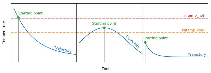
initemp_cold= 8 WinNet is able to start at a given temperature and evolve the electron fraction with weak reactions until the system falls out of NSE. This temperature determines the start of the calculation. If it is higher than the maximum temperature of the trajectory, the calculation will start at the maximum temperature that is larger than initemp_cold.
initemp_hot= 10 Initial stepsize of the calculation.
initial_stepsize= 1e-15 Interpolation method that is used for the interpolation of temperature and density when trajectory_mode is set to "from_file". All interpolations are performed in lin-log space. The interp_mode parameter is a integer that translates to
| Value | Interpolation |
|---|---|
| 1 | Linear |
| 2 | Cubic |
| 3 | Akima |
| 4 | modified Akima |
| 5 | PCHIP |
For an example trajectory the interpolations look as follows:
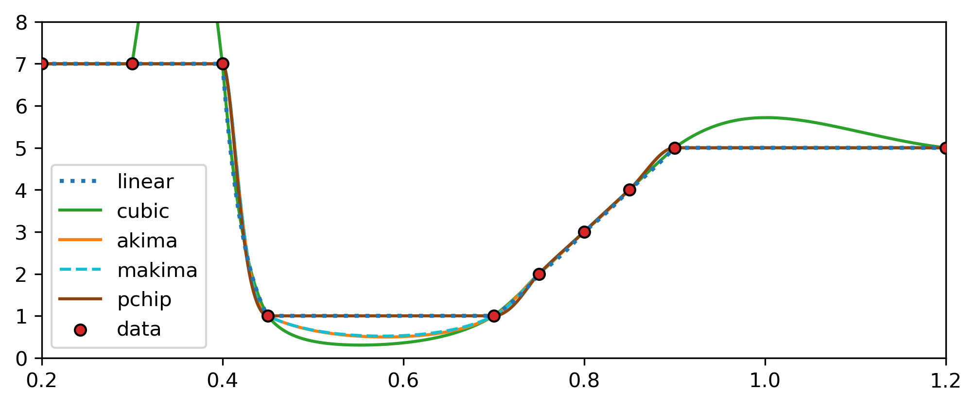
The default interpolation is the PCHIP.
interp_mode= 3 Mandatory file that contains the partition functions and the mass excess of the contained isotopes. The second line of this file contains the temperature grid points for the values of the partition function. For example the line 010015020030040050060070080090100150200250300350400450500600700800900100 is translated into (0.10, 0.15, 0.20, 0.30,..., 8.00, 9.00, 10.0) GK. After the second line, the file contains a list of isotopes, where the last isotope of the list is contained twice. An example file looks like:
   010015020030040050060070080090100150200250300350400450500600700800900100
       n
       p
       p
       n       1.000   0   1   0.5     8.071
        1.00     1.00     1.00     1.00     1.00     1.00     1.00     1.00
        1.00     1.00     1.00     1.00     1.00     1.00     1.00     1.00
        1.00     1.00     1.00     1.00     1.00     1.00     1.00     1.00
       p       1.000   1   0   0.5     7.289
        1.00     1.00     1.00     1.00     1.00     1.00     1.00     1.00
        1.00     1.00     1.00     1.00     1.00     1.00     1.00     1.00
        1.00     1.00     1.00     1.00     1.00     1.00     1.00     1.00
where n is the name, 1.000 the mass number, 0 the atomic number, 1 the neutron number, 0.5 the spin of the ground state and 8.071 the mass excess of the isotope in MeV. The mass excess is defined as
\[ \Delta = mc^2-Auc^2 \]
where \(m\) is the mass of the atom (i.e., includes the electron rest mass), \(c\) is the speed of light, \(A\) is the mass number of the nuclide, and \(u\) is the atomic mass unit. As the atomic mass unit \(u\) is defined as 1/12 of the mass of a \(^{12}\)C nuclide, the mass excess of this isotope is per definition zero.
Below this line, the values of the partition functions for the temperature grid that was given in the first line are listed. The difference between a winvn and winvne file from JINA Reaclib is the format of the partition functions. It can be written with floats (winvn) and in scientific notation (winvne). WinNet is able to read both formats.
isotopes_file= "@WINNET@/data/winvne_v2.0.dat" Flag whether the rates contained in weak_rates_file are used or not. Possible values are:
| iwformat | Description |
|---|---|
| 0 | no theoretical weak rates are used. |
| 1 | tabulated theoretical weak rates are used. |
| 2 | log(ft) theoretical weak rates are used. |
The default file rateseff.out is tabulated logarithmically and is taken from Langanke & Martinez-Pinedo 2001. Therefore, the flag 1 is deprecated and will not produce correct results when using the default file.
iwformat= 2 Flag whether the weak rates rates are interpolated bilinear or bicubic. Possible values are:
| iwinterp | Description |
|---|---|
| 0 | bilinear interpolation |
| 1 | bicubic interpolation |
iwinterp= 0 Constant value or function for electron-neutrino luminosities in erg \(\,\)s \(^{-1}\). Only used when neutrino_mode is set to "analytic".
Le= 2e51 Constant value or function for electron-antineutrino luminosities in erg \(\,\)s \(^{-1}\). Only used when neutrino_mode is set to "analytic".
Lebar= 2e51 Constant value or function for the summed value of muon-neutrino and tau-neutrino luminosities in erg \(\,\)s \(^{-1}\). Only used when neutrino_mode is set to "analytic" and nuflag is 4 or 5.
Lx= 2e51 * 2 Constant value or function for the summed value of muon-antineutrino and tau-antineutrino luminosities in erg \(\,\)s \(^{-1}\). Only used when neutrino_mode is set to "analytic" and nuflag is 4 or 5.
Lxbar= 2e51 * 2 Main output of the network. This parameter determines the frequency at which this output is given. It contains: iteration, time in \(\mathrm{s}\), temperature in \(\mathrm{GK}\), density in \(\mathrm{g \, cm^{-3}}\), electron fraction, abundance of neutrons, abundance of protons, abundance of alpha particles, abundance of elements with \(A\le 4\), abundance of elements with \(A>4\), average atomic number, average mass number, entropy in \(\mathrm{k_B/baryon}\), and the average neutron separation energy if the parameter calc_nsep_energy was set to `‘yes’'. This output is stored into the file mainout.dat. An example file looks like:
    # 1:iteration 2:time[s], 3:T[GK], 4:rho[g/cm3], 5:Ye
    # 6:R[km], 7:Y_n, 8:Y_p, 9:Y_alpha, 10:Y_lights
    # 11:Y_heavies 12:<Z> 13: 14:entropy [kB/baryon] (15:Sn [MeV])
       0  0.0000000000000000E+00   1.0964999999999998E+01   8.7095999999999795E+12   3.4880000000001680E-02   4.9272999999999975E+01   8.7430471311642388E-01   1.8154340816658842E-15   1.8313910002116333E-13   8.4293473893924100E-09   1.6154109228777289E-03   3.9820982195819934E-02   1.1416565996507526E+00   9.4638587929828290E-03
      10  4.0940000000000001E-09   1.0965038071994945E+01   8.7093701186135752E+12   3.4880006806212963E-02   4.9273176232580205E+01   8.7430472419630612E-01   1.8157922458135375E-15   1.8317495847108614E-13   8.4302150496944692E-09   1.6154086944791908E-03   3.9820989563731306E-02   1.1416565881127740E+00   9.4639764072160116E-03
...mainout_every= 15 Mandatory file that contains a list of all isotopes that are used in the network. Each column of the file should contain 5 characters and the names of the isotopes should be orientated to the right. Example:
    n
    p
    d
    t
   he3
   he4
   he6
   li6
   li7
   li8
   li9
...net_source= "@WINNET@/data/sunet_complete"Path to a file that contains the information of the average neutrino energy that gets produced by \( \beta \)-decays. This is only relevant if heating_mode is greater than 0. An example of the file could look like:
...
 al34     4.803857E+00
 al35     6.072946E+00
 al37     5.639200E+00
 si25     4.794861E+00
...
where the first column is the decaying nucleus and the second column the average energy of the neutrinos in MeV that get released by the decay.
neutrino_loss_file= "nuloss_file.dat"Flag to indicate if the neutrino quantities (i.e., luminosities and energies) should get read from a trajectory file or from an analytic expression. Possible values are "analytic" or "from_file".
neutrino_mode= "from_file"Fission fragment probabilities of neutron induced fission. For fissflag equal to 3 and 4, the file format has to be as given in Mumpower et al. 2020. An example is given by:
     93  220  574
     0 0 0
     019  048  1.96607e-06
     020  048  2.24289e-05
     020  049  1.88041e-05
     020  050  7.65944e-06
     020  051  1.62040e-06
     021  048  1.17847e-05
     021  049  3.62928e-05
The first line contains the Z, A and number of the fissioning nucleus. The next line is a dummy line. Then followed by Z, A and the yield Y(Z,A). Note that \(\sum Y(Z,A) \cdot A \) should be the mass number of the parent nucleus. Furthermore, \(\sum Y(Z,A) = 2\).
nfission_file= "@WINNET@/data/NFISSION"Maximum amount of iterations within the Newton-Raphson algorithm. This parameter is only used in case that solver is set to 0. The default value is 3.
nr_maxcount= 10Minimum amount of iterations within the Newton-Raphson algorithm. This parameter is only used in case that solver is set to 0. The default value is 2.
nr_mincount= 1Exit accuracy of the Newton-Raphson algorithm. This parameter is only used in case that solver is set to 0. The default value is 1e-5.
nr_tol= 1e-7Since WinNet uses implicit numerical methods, a root finding algorithm must be applied. Here, it is the Newton-Raphson method. With the parameter nrdiag_every you can check the convergence of this root finding algorithm. If the frequency is \(>0\) a file nrdiag.dat will be created, containing iteration, time in \(\mathrm{s}\), temperature in \(\mathrm{GK}\), a counter that indicates how often the step size was corrected, a counter for the number of steps that where necessary for the Newton-Raphson algorithm to achieve convergence, the time step in \(\mathrm{s}\), an error of the mass conservation, the maximal change of an abundance in the iteration, the name of the isotope that determined the time step, and the abundance of this isotope. An example file looks like:
 # Newton-Raphson diagnostic output
 # 1 : global iteration count (cnt)
 # 2 : global time [s]
 # 3 : temperature T9 [GK]
 # 4 : adapt stepsize loop counter (k)
 # 5 : NR loop counter (nr_count)
 # 6 : global timestep [s]
 # 7 : mass conservation error
 # 8 : maximal abundance change (eps)
 # 9 : most rapidly evolving isotope (epsl)
 # 10: abundance of the isotope epsl, y(epsl)
       0   5.20740000000E-22   7.42450000000E+00    0    1   5.20740000000E-22   9.32587340685E-15   2.22044604925E-16 cl42   2.43899441583E-08
       0   5.20740000000E-22   7.42450000000E+00    0    2   5.20740000000E-22   9.32587340685E-15   2.22044604925E-16  s40   2.73320077046E-08
       1   1.56220000000E-21   7.42450000000E+00    0    1   1.04146000000E-21   9.32587340685E-15   2.22044604925E-16  he4   3.13811866442E-03
       1   1.56220000000E-21   7.42450000000E+00    0    2   1.04146000000E-21   9.32587340685E-15   2.22044604925E-16 mg30   1.57736344914E-10
...nrdiag_every= 10Since weak reactions are changing the electron fraction during the phase of nuclear statistical equilibrium, the composition changes as well. This parameter sets the frequency of recalculating the NSE composition, which can have an impact on the evolution of the electron fraction. If it is set to zero, the composition will be calculated only when entering the regime of NSE and when leaving it. The default value is 1, i.e., always calculate NSE.
nse_calc_every= 1 Minimum temperature in GK when descending from nse_descend_t9start to the desired temperature. If smaller temperatures are necessary, an error is raised. The default value is 1d-16.
nse_delt_t9min= 100 The nuclear statistical equilibrium is calculated as in, e.g., Hix & Thielemann 1999. For numerical reasons it is advantageous to start with a high temperature and iterate to lower temperatures, using the result of the old temperature as input value for the new temperature. This parameter determines the highest temperature in GK for this iteration. A default value of this parameter is \(100\, \mathrm{GK}\).
nse_descend_t9start= 100 Maximum amount of iterations to bring the NSE solver to convergence. The default value is 25.
nse_max_it= 50 Convergence criteria within the solving scheme of the NSE calculation. The default value is 1d-6.
nse_nr_tol= 1d-4 Flag to decide which solver to use to determine the NSE composition. Possible options are:
| nse_solver | Solver |
|---|---|
| 0 | Newton-Raphson |
| 1 | Powell's hybrid method |
Hereby, Powell's hybrid method uses the MINPACK-I package downloaded from here. The default value is 0.
nse_solver= 1 Path to a file that contains neutron separation energies. This file is only relevant if calc_nsep_energy has been enabled. An example of a file could look like:
   ...
   8   6  14  2.3176000E+01
   8   7  15  1.3222000E+01
   8   8  16  1.5664000E+01
   8   9  17  4.1433000E+00
   8  10  18  8.0443700E+00
   8  11  19  3.9553000E+00
   8  12  20  7.6073700E+00
   8  13  21  3.7373700E+00
   8  14  22  6.7613700E+00
   9   8  17  1.6800000E+01
   9   9  18  9.1500000E+00
   9  10  19  1.0432000E+01
   9  11  20  6.6013000E+00
   ...
where the first column is the amount of protons, the second the amount of neutrons, the third the amount of nucleons, and the fourth one the neutron separation energy.
nsep_energies_file= frdm_sn.dat Temperature at which the nuclear reaction network switches from NSE evolution to the full network evolution. This temperature is given in GK.
nsetemp_cold= 5 Due to nuclear heating, it can happen that the network bounces between NSE evolution and network evolution. To prevent this, two temperatures can be given and the transition between NSE and the network can be different from the transition between the network and NSE.
nsetemp_hot= 8 File to specify channels for neutrino reactions. This file is only used for nuflag 3-5. The file follows the format of Sieverding et al.2018. An example looks like:
   id    type     particle emission


   001 nue    (cc)  0p 0n 0a
   002 nue    (cc)  1p 0n 0a
   003 nue    (cc)  0p 1n 0a
   004 nue    (cc)  0p 0n 1a
   005 nue    (cc)  2p 0n 0a
   ...
where the type "cc" stands for charged current and "nc" for neutral current. The particle emission is the number of particles emitted in the reaction (p: protons, n: neutrons, a: alphas). The first line is a header line and is ignored. The original file can be found in the supplemental material in Sieverding et al.2018.
nuchannel_file= nu_channels Parameter to specify the treatment of neutrino reactions. Possible values are:
| nuflag | Description | Format | Necessary other parameters |
|---|---|---|---|
| 0 | No neutrino reactions. | - | - |
| 1 | Neutrino captures of \(\nu_e\), \(\bar{\nu_e}\) on nucleons. | - | nunucleo_rates_file |
| 2 | \(\nu_e\), \(\bar{\nu_e}\) on nucleons and heavy nuclei (only charged current reactions). | Sieverding et al.2018. | nunucleo_rates_file, nuchannel_file, nurates_file |
| 3 | \(\nu_e\), \(\bar{\nu_e}\) on nucleons, neutral current reactions on heavy nuclei. | Sieverding et al.2018. | nunucleo_rates_file, nuchannel_file, nurates_file |
| 4 | \(\nu_e\), \(\bar{\nu_e}\) on nucleons, charged and neutral current reactions on heavy nuclei. | Sieverding et al.2018. | nunucleo_rates_file, nuchannel_file, nurates_file |
If neutrinos are included, neutrino reaction rates are read from the files nunucleo_rates_file, nuchannel_file, or nurates_file (see table which parameter is necessary). In case of neutral current reactions included (nuflag 3 or 4), also the luminosities and temperatures of muon/tau neutrinos have to be given either in the trajectory or in analytic form.
nuflag= 1 Output frequency for energy that is added or lost from the system. If this parameter is greater than one, a file called nu_loss_gain.dat will be created. Hereby, there is a distinction between energy lost by neutrinos that are created in beta-decay, energy lost by thermal neutrinos, and energy added to the system by neutrino reactions. An example file could look like:
  # File containing the neutrino loss/gain for the nuclear heating.
  # Negative values mean that energy is added to the system.
  # Neutrino energies are given in MeV/baryon/s.
  #         time[s]                 T[GK]            rho[g/cm3]                 R[km]              nu_total ...
        1.64334E-04           1.00000E+01           7.05312E+07           3.02337E+02           0.00000E+00 ...
        1.64334E-04           1.00000E+01           7.05312E+07           3.02337E+02          -2.77996E+01 ...
        1.64334E-04           1.00000E+01           7.05312E+07           3.02337E+02          -2.77996E+01 ...
        1.64334E-04           1.00000E+01           7.05312E+07           3.02337E+02          -2.77996E+01 ...
        1.64334E-04           1.00000E+01           7.05312E+07           3.02337E+02          -2.77996E+01 ...
...nu_loss_every= 1 Specifies the time limit in seconds for neutrino reactions. Neutrino interactions will be disabled after this duration. A value of -1 keeps neutrino reactions active indefinitely (default). Note that this can be necessary as WinNet keeps the neutrino quantities constant after the trajectory has ended.
nu_max_time= 10.0Specifies the minimum neutrino luminosity in erg/g/s required to consider neutrino reactions. Neutrino interactions will only be included if the luminosity exceeds this threshold. A value of 1 erg/g/s is used by default.
nu_min_L= 1e30Specifies the minimum neutrino temperature in MeV required to consider neutrino reactions. Neutrino interactions will only be included if the temperature exceeds this threshold. A value of 1 MeV is used by default.
nu_min_T= 1.0Path to a file, containing neutrino capture rates on protons and neutrons. The file contains tabulated values of the rates, using a neutrino temperature grid of \(2.8, 3.5, 4.0, 5.0, 6.4, 8.0, 10.0 \,\mathrm{MeV}\). An example of this file is given by (located in data/neunucleons.dat):
         n    p                             nen
 12.39     18.64     23.89     36.38     58.36     89.96    139.28
 13.67     17.23     19.77     24.87     32.00     40.17     50.37
         p    n                            nebp
  7.11     11.27     14.76     22.94     36.79     55.56     82.64
 14.58     17.96     20.37     25.13     31.71     39.12     48.22
The first line of the file indicates the reaction, similar to the reaclib format. The next line indicates the tabulated cross section and the line below the average energy of the absorped neutrino. The data is calculated as in Burrows et al. 2006 with weak magnetism corrections as in Horowitz 2002.
nunucleo_rates_file= "@WINNET@/data/neunucleons.dat" Path to a file, containing neutrino reactions. These reactions can be charged current or neutral current reactions. They use a neutrino temperature grid of \(2.8, 3.5, 4.0, 5.0, 6.4, 8.0, 10.0 \,\mathrm{MeV}\). The format comes from Sieverding et al.2018. An example of the file looks like:
    000  Z = 2    A = 4   channels:  6
    002  1.099778E-03  7.960983E-03  2.308440E-02  1.163089E-01  5.736357E-01  2.100826E+00  6.820661E+00
    023  1.145175E-03  7.713879E-03  2.115540E-02  9.541441E-02  4.077819E-01  1.295820E+00  3.633845E+00
    ...
Here the first line contains the atomic number, the mass number and the amount of reactions. The second line contains the channel specified in the channel file (see nuchannel_file) followed by the reaction rates. The reaction rates are tabulated on a (neutrino) temperature grid of Tnu (MeV) = 2.800 3.500 4.000 5.000 6.400 8.000 10.000. The file can be also downloaded in the supplemental material of Sieverding et al.2018.
nurates_file= "@WINNET@/data/nucross.dat" Parameter to specify a brief output. If you start WinNet by using the terminal, this output will be shown in the terminal. It consists of short status messages (e.g., the network size), the iteration, time, temperature, density, and entropy.
       WinNet - Nuclear reaction network
      ===================================


    Option                                   :      Value     Unit
    --------------------------------------------------------------
    Network size                             :       6545
    Amount reaclib rates                     :      70565
    Amount fission rates                     :       4301
    Total number of fission neutrons         :      17100
    Amount weak (ffn) rates                  :        212
    Total reactions after merge              :      74976
    Thermodynamic trajectory                 :  from file
    Starting index                           :          1
    Expansion velocity:                      :   4.00E+04   [km/s]
    Initial abundance source                 :        NSE
    Evolution mode                           :        NSE
    Initial entropy                          :   9.46E-03 [kB/nuc]


    #-- 1:it 2:time[s] 3:T9[GK] 4:rho[g/cm3] 5:entropy[kB/baryon]
    0  0.0000000E+00 10.9650000  8.7096000E+12    0.0094639
    1  2.0000000E-12 10.9650000  8.7095999E+12    0.0094639
... out_every= 10 File to a previously created folder with reaction rate and nuclear data. For more information see the description of the parameter use_prepared_network.
prepared_network_path= network_data/ Path to a mandatory reaction rate file (Cyburt et al.2010). It contains reaction rates in order to solve the reaction network. WinNet is only able to handle the Reaclib 1 (R1) original format without chapter 9, 10, 11. All rates in the REACLIB database are fitted by the function
\[ \lambda = \mathrm{exp} \left[ a_0 + \sum \limits _{i=1} ^5 a_i T_9 ^{\frac{2i-5}{3}} + a_6 \, \mathrm{ln} T_9 \right]. \]
An exemplary entry for on reaction rate is given below. The reactions are divided into different chapters, which is given by the first number in a single line (in the example below, it is chapter "4"). Afterwards, the participating nuclei are indicated, followed by the literature source of the reaction (see here), a flag for resonant and one for reverse rates ("r" and "v"), and the Q-value of the reaction. The next lines contain the \(a_i\) parameters for the fit function.
   Example reaclib_file:
   ...
   4
   ...
            n ge65 ge66                       talyr     1.32001e+01
    1.851912e+01 0.000000e+00 0.000000e+00-1.731299e+00
    1.979346e+00-1.136181e+00-1.560352e-01 2.967128e-01-2.840840e-02
   ...
It is possible to replace some of the weak reaction rate files by theoretical ones as described in the parameter weak_rates_file. A more extensive explanation of the reaclib file format is given here.
reaclib_file= "@WINNET@/data/20140416defaultno910" Boolean parameter that specifies whether the initial composition should be read from the file seed_file.
read_initial_composition= yes Analytic density evolution. This expression is only evaluated when the parameter trajectory_mode is set to "analytic".
rho_analytic= (5e-1*cos(x)+1)*1e6+sin(pi) Analytic radius evolution. This expression is only evaluated when the parameter trajectory_mode is set to "analytic".
Rkm_analytic= ln(x)+1 Determines the prescription of coulomb corrections. Screening accounts for the change of the coulomb potential of the nucleus by electrons and has therefore an impact on the reaction rates (and NSE). Screening corrections are taken into account in NSE as well as in lower temperature regimes. Possible values are:
| screening_mode | Description |
|---|---|
| 0 | No corrections |
| 1 (default) | Corrections as in Kravchuk & Yakovlev 2014 |
screening_mode = 0 Optional file to specify the composition. The format of this file can be specified by seed_format . If the sum over all mass fractions is not exactly one, the initial composition is renormalized.
seed_file = @WINNET@/data/Example_data/seed The columns and structure of the seed file is determined by the user defined parameter parameter_class::seed_format. The default seed format is given by: "name X" . This format will assume a file that looks like:
    # Name X
    #---------------
    n    0.0000e+00
    p    2.5000e-05
    he4  5.0000e-05
    ...
Another example for seed format "A Z X skip" looks like:
       1   0    2.000000e-01  unimportant
       1   1    1.000000e-01  unimportant
      12   6    2.000000e-01  unimportant
      16   8    3.000000e-01  unimportant
      40  20    1.500000e-01  unimportant
      98  48    0.500000e-01  unimportant
Possible column names are:
| Column value | Description |
|---|---|
| A | Mass number |
| Z | Atomic number |
| N | Neutron number |
| Y | Abundance |
| X | Mass fraction |
| Name | Nucleus name |
| skip | Skip column |
The first rows of the seed file will be skipped if they start with "#" or are blank.
seed_format = "A Z Y" File that contains the fission fragment probabilities of spontaneous fission in case that fissflag is set to 4 and fission_frag_spontaneous is set to 3. An example is given by:
    93  220  574
   0 0 0
   019  048  1.96607e-06
   020  048  2.24289e-05
   020  049  1.88041e-05
   020  050  7.65944e-06
   020  051  1.62040e-06
   021  048  1.17847e-05
   021  049  3.62928e-05
   021  050  5.43032e-05
   ...
Here, the first line specifies the fissioning nucleus (atomic number, mass number) and the amount of fission fragments (39). The second line is a dummy line which is not used within WinNet. From the third line onwards, the fission fragments are specified (atomic number, mass number) together with their yield. The third column therefore adds up to one over all fragments. This file is read only when fissflag was set to four. Noe that the following must hold:
\[ \sum Y(Z,A)\cdot A = A_\text{fiss} \]
with the mass number of the fissioning nucleus \( A_\text{fiss}\). Otherwise an error is raised.
sfission_file= "@WINNET@/data/SFISSION"Frequency of an output of all abundances. This output will be stored in the sub folder of the run snaps/.
       time    temp    dens
      6.00000000000000E-03   3.00000000000000E-07   1.00000000000000E+00
        nin     zin       y       x
     1    0     9.99993224403019E-03   9.99993224403019E-03
     0    1     9.90000067755970E-01   9.90000067755970E-01
....snapshot_every = 10 Path to a file for providing points in time in days for custom snapshots. This file is only used if custom_snapshots are enabled. The file:
   0.04166666
   1
   365
   3650
   36500
creates a snapshot after one hour, one day, one year, \(10\) years, and \(100\) years.
snapshot_file= "@WINNET@/data/Example_data/Example_MRSN_nup_process_obergaulinger/custom_snapshots.dat" WinNet contains different solver. With the parameter solver you specify which solver should be used. Possible values are:
| solver | Description |
|---|---|
| 0 | Implicit euler. |
| 1 | Gear's method. |
solver = 1 Initial time in seconds for analytic trajectory mode. This time is only assumed for constant hydrodynamic conditions. Otherwise the calculation starts at the point where the temperature is lower than initemp.
t_analytic = 1e-3 Analytic temperature evolution in GK. This expression is only evaluated when the parameter trajectory_mode is set to "analytic".
T9_analytic = sin(x)+10**(-5)*exp(-x+20)+4-10**(-2)*x File with tabulated rates that is used when use_tabulated_rates is turned on. The file looks similar as a reaclib_file, i.e., it is also splitted into chapters, has a source string, and a Q-value. An example is shown below:
   4
   ....
          c12  c12 mg24                       tabln     0.00000e+00
   0.000E+00 0.000E+00 0.000E+00 0.000E+00 0.000E+00 1.634E-72 2.768E-52 1.768E-42 ...
          c12  o16 si28                       tabln     0.00000e+00
   0.000E+00 0.000E+00 0.000E+00 0.000E+00 0.000E+00 0.000E+00 0.000E+00 0.000E+00 ...
          o16  o16  s32                       tabln     0.00000e+00
   0.000E+00 0.000E+00 0.000E+00 0.000E+00 0.000E+00 0.000E+00 1.845E-90 1.594E-74 ...
   ....
In contrast to Reaclib, it has one long line of a rate tabulation. The temperature grid points are given by: 1.0d-4, 5.0d-4, 1.0d-3, 5.0d-3, 1.0d-2, 5.0d-2, 1.0d-1, 1.5d-1, 2.0d-1, 2.5d-1, 3.0d-1, 4.0d-1, 5.0d-1, 6.0d-1, 7.0d-1, 8.0d-1, 9.0d-1, 1.0d+0, 1.5d+0, 2.0d+0, 2.5d+0, 3.0d+0, 3.5d+0, 4.0d+0, 5.0d+0, 6.0d+0, 7.0d+0, 8.0d+0, 9.0d+0, 1.0d+1 GK.
tabulated_rates_file = tabl_rates.dat File with a temperature grid that is used for all tabulated rates. In case 'default' is given, the default temperature grid that is given by 30 points: 1.0d-4, 5.0d-4, 1.0d-3, 5.0d-3, 1.0d-2, 5.0d-2, 1.0d-1, 1.5d-1, 2.0d-1, 2.5d-1, 3.0d-1, 4.0d-1, 5.0d-1, 6.0d-1, 7.0d-1, 8.0d-1, 9.0d-1, 1.0d+0, 1.5d+0, 2.0d+0, 2.5d+0, 3.0d+0, 3.5d+0, 4.0d+0, 5.0d+0, 6.0d+0, 7.0d+0, 8.0d+0, 9.0d+0, 1.0d+1 GK is used. This parameter is only used in case use_tabulated_rates is set to 'yes'. An example file could look like:
1d-3 1d-2 1d-1 1d0 2d0 3d0 4d0
where each column contains a temperature in GK. Note that the tabulated rates given in tabulated_rates_file must have the same number of entries.
tabulated_temperature_file = default The reaction rates are only valid above \(10^{-2}\) GK. Therefore the parameter temp_reload_exp_weak_rates specifies the temperature at which the rates are replaced with rates specified in the reaclib_file. This temperature is only important if iwformat is greater than 0.
temp_reload_exp_weak_rates = 1d-2 The termination criterion can be set with the parameter termination_criterion. Possible values are:
| termination_criterion | Description |
|---|---|
| 0 | terminate simulation in the end of trajectory. |
| 1 | terminate after final time is reached. |
| 2 | terminate after final temperature is reached. |
| 3 | terminate after final density is reached. |
The final values can be set by the parameters final_time, final_temp, final_dens.
termination_criterion = 0 Parameter to specify the frequency of the average timescales of each reaction type. These timescales are calculated as in Arcones et al. 2012 (Eq. 1-6). The (p,gamma) timescale is given by e.g.,
\[ \tau_{p\gamma} = \left[ \frac{\rho Y_p}{Y_h}N_A \sum \langle \sigma \nu \rangle_{p,\gamma}(Z,A)Y(Z,A) \right]^{-1} \]
The timescales are stored to the file timescales.dat, containing the timescales in \(\mathrm{s}^{-1}\) of the reaction types. An example file looks like:
   # time[s]     Temperature [GK]     tau_ng [s]     tau_gn [s]     tau_pg [s]     tau_gp [s]     tau_np [s]     tau_pn [s]     tau_an [s]     tau_na [s]     tau_beta [s]     tau_alpha [s]     tau_nfiss [s]     tau_sfiss [s]     tau_bfiss [s]
    1.1130000000000000E+00    9.1821750000000009E+00    0.0000000000000000E+00    0.0000000000000000E+00    0.0000000000000000E+00    0.0000000000000000E+00    0.0000000000000000E+00    0.0000000000000000E+00    0.0000000000000000E+00    0.0000000000000000E+00    1.2642767370327558E+01    2.9487624276191804E+00    0.0000000000000000E+00    0.0000000000000000E+00    0.0000000000000000E+00
    1.1220000000000001E+00    8.2638489999999951E+00    0.0000000000000000E+00    0.0000000000000000E+00    0.0000000000000000E+00    0.0000000000000000E+00    0.0000000000000000E+00    0.0000000000000000E+00    0.0000000000000000E+00    0.0000000000000000E+00    1.0557999180036711E+02    2.5923655028366777E+01    0.0000000000000000E+00    0.0000000000000000E+00    0.0000000000000000E+00
    1.1247618491767180E+00    7.9904974735555152E+00    9.5690472538317728E-13    5.3150487750907188E-11    7.4419112944811684E-10    9.8479480155439862E-08    1.9792689873245490E-12    1.9444248037144314E-12    4.8686627517806918E-10    3.9657685448682009E-12    1.4600540103519526E+01    5.2634156341152767E+01    0.0000000000000000E+00    0.0000000000000000E+00    0.0000000000000000E+00
...timescales_every = 5 Maximum allowed difference of temperature or density within one timestep. E.g., if set to 0.05, the temperature is maximum allowed to change by 5 percent. In case that nuclear heating is enabled, only the density is restricted.
timestep_hydro_factor = 0.05 Maximum allowed ratio of the new time step and the old time step, \(h_{\mathrm{new}} / h_{\mathrm{old}}\).
timestep_max = 2 The time step of implicit Euler is determined by:
\[ h_{\mathrm{new}} = \eta \cdot \mathrm{min_i}\left( |\frac{Y_i}{\dot{Y_i}}| \right), \]
where \(\eta = \mathrm{timestep\_factor}\), which is the same as the estimated maximal change of the most rapidly evolving nucleus, because from
\[ \left| \dot{Y}\right| = \left|\frac{Y(t+h) - Y(t)}{h}\right| \]
and
\[ \eta = \left|1-\frac{Y(t+h)}{Y(t)} \right| \]
follows:
\[ \left|\dot{Y}\right| = \left| \frac{(1 - \eta ) \cdot Y(t) - Y(t)}{h}\right| \Rightarrow h = \eta \left|\frac{Y(t)}{\dot{Y}(t)}\right|. \]
timestep_factor = 0.1 Including all nuclei into the determination of the time step, even nuclei with very small abundances would make the time step infinitesimal small. The parameter timestep_Ymin sets a lower bound for the abundance of a nucleus to contribute to the time step.
timestep_Ymin = 1e-10 This parameter can either have the value yes'' orno''. If it is set to `‘yes’', the calculation will be limited by the one of the given trajectory. In other words, in case a timestep would exceed the hydro grid point, it will instead be limited to the hydro grid.
timestep_traj_limit = no Integer parameter that specifies if top contributor to the nuclear energy generation should get printed to the file toplist.dat . An example of the file is given by:
#                               Top nuclear energy producers for each reaction given in erg/g/s
#    Time[s]   Etot[erg/g/s]    Reaction_1                       Reaction_2                       Reaction_3                       Reaction_4                       Reaction_5                       Reaction_6                       Reaction_7           ...
  1.1039E+00      0.0000E+00    he4 => t + n                     he4 => he3 + p                   p => n                           p => n                           c12 => n11 + n                   c12 => be11 + p                  c12 => b8 + he4      ...
  1.1039E+00      1.0639E+20    n => p                           n => p                           p + p => d                       he6 => li6                       p + p => d                       b12 => c12                       li8 => he4 + he4     ...
    ...
This file lists the reactions contributing most to the generated energy (positively and negatively) as well as the value of the energy in erg/g/s. For this list, fission reactions are not considered. Additionally, the file lists the isotopes and energy of the most changing isotopes (positively and negatively). Note that in the above example, "n => p" can be a neutrino reaction, beta decay, or positron capture. The energy of the reactions are calculated, for the example of a two-body reaction, by
\[ \dot{E} = C \langle \sigma v \rangle \rho Y_1 Y_2 Q \]
where C is the double counting factor, \( \langle \sigma v \rangle \) is the cross section of the reaction, \( \rho \) the density, Y the abundance, and Q is the energy released in the reaction. The energy released by isotope is calculated by
\[ \dot{E} = -M_\mathrm{exc} (Y_t-Y_\mathrm{t-1})/h \]
with the mass excess \( M_\mathrm{exc} \), the abundance of the current time step \(Y_t\), the abundance \(Y_\mathrm{t-1}\), and the time step h.
With python one can use the pandas package to read this file with the following lines:
import pandas as pd
df = pd.read_csv("toplist.dat",sep="\s{2,}",skiprows=2,header=None)
top_engen_every = 10 One can track the evolution of abundances of individual nuclei. If the parameter is larger than zero, a file called tracked_nuclei.dat will be created in the run folder. For this a path of a valid file must be given for the parameter track_nuclei_file.
   # time[s]                    Y(  ni56 )                  Y(  ti44 )                  Y(  ca48 )
    4.4479893740127485E-01      0.0000000000000000E+00      0.0000000000000000E+00      3.7857260959653261E-23
    4.4536148263636188E-01      0.0000000000000000E+00      1.2167485211212250E-24      1.4314310210168970E-21
    4.4596649436475339E-01      0.0000000000000000E+00      9.9175184259232737E-24      2.7418559494841269E-20
... track_nuclei_every = 10 When specifying track_nuclei_every larger than zero, this parameter should be set to a path to a valid file, containing names of nuclei you want to track. The format of this file should be the same as given in net_source. An example could be:
    c13
   ti44
ni56 track_nuclei_file = @WINNET@/data/trackfile.dat Path to a trajectory file, matching the given format specified in trajectory_format. This file will only get read in case trajectory_mode was set to "from_file".
trajectory_file = "@WINNET@/data/trajectories/trajectory_00001_winnet.dat" The columns and structure of the file is determined by the user defined parameter parameter_class::trajectory_format. The default trajectory format is given by: "time temp dens rad ye" . This format will assume a file that looks like:
    #time[s], T9[GK], density[g/cm^3], R[km], Ye
    #--------------------------------------------
    0.0000e+00 1.0965e+01 8.7096e+12 4.9273e+01 0.03488
    2.5000e-05 9.9312e+00 7.4131e+12 5.0361e+01 0.03488
    ...
A more complex format, "time:ms x y z log_dens log_temp:K ye" , would assume a file like:
    t [ms]       x[km]       y[km]      z[km]      log(rho[cgs]) log(T[K])   Ye
    ----------------------------------------------------------------------------------
     0.0000E+00  0.1051E+02  0.3774E+01 -0.4538E+01  0.1364E+02  0.1016E+02  0.1604E-01
     0.2521E-01  0.1046E+02  0.4724E+01 -0.4541E+01  0.1363E+02  0.1060E+02  0.1604E-01
    ...
Neutrino luminosities and energies are also read here. A format could look like: "time temp dens rad ye lnu lanu tnu tanu" .
Possible column names are:
| Column value | Description |
|---|---|
| time | The time (s) of the trajectory |
| temp | The temperature (GK) of the trajectory |
| dens | The density (g/ccm) of the trajectory |
| rad | The radius (km) of the trajectory |
| x,y,z | x, y, and z coordinates (km) of the trajectory |
| ye | The electron fraction |
| lanue | Anti-electron neutrino luminosities (erg/s) |
| lnue | Electron neutrino luminosities (erg/s) |
| tanue | Electron anti-neutrino temperatures (MeV) |
| tnue | Electron neutrino temperatures (MeV) |
| eanue | Electron anti-neutrino energies (MeV) |
| enue | Electron Neutrino energies (MeV) |
| lanux | Summed muon and tau anti-neutrino luminosities (erg/s) |
| lnux | Summed muon and tau neutrino luminosities (erg/s) |
| tanux | Muon and tau anti-neutrino temperatures (MeV) |
| tnux | Muon and tau neutrino temperatures (MeV) |
| eanux | Muon and tau anti-neutrino energies (MeV) |
| enux | Muon and tau neutrino energies (MeV) |
| skip | skip a column |
trajectory_format = "time temp dens rad ye lnu lanu tnu tanu" The trajectory mode determines the source of temperature and density used in the network calculation. Possible values are:
| trajectory_mode | Description |
|---|---|
| "from_file" | Follow a trajectory. |
| "analytic" | Get temperature and density from an analytic formula |
When choosing "from_file", two additional parameters have to be given. One specifies the path to the trajectory file and the other parameter specifies the format of this file.
trajectory_mode = "from_file" Use additional alpha-decays that are given in alpha_decay_file. The default file was calculated via the Viola-Seaborg formula. Additional alpha-decays can either replace existing ones in reaclib or only complement the reaclib rates. Via the Viola-Seaborg formula the alpha-decay rates can be empirically approximated by
\[ \log_{10}T_\alpha = (aZ + b)Q_\alpha^{-0.5} + (cZ + d)+h_{log} \]
with certain fit parameters. The parameters are chosen as follows:
| a | b | c | d | |
|---|---|---|---|---|
| \(Z>82\), \(N>126\) | 1.64062 | -8.54399 | -0.19430 | -33.9054 |
| \(Z>82\), \(82<N\le126\) | 1.71183 | -7.50481 | -0.25315 | -30.7028 |
| \(50<Z\le 82\), \(82<N\le126\) | 1.70875 | -7.52265 | -0.25153 | -30.8245 |
| \(50<Z\le 82\), \(50<N\le82\) | 1.71371 | -7.34226 | -0.24978 | -30.6826 |
| h1 | h2 | h3 | h4 | |
| \(Z>82\), \(N>126\) | 0 | 0.8937 | 0.5720 | 0.9380 |
| \(Z>82\), \(82<N\le126\) | 0 | 0.0476 | 0.1214 | 0.3933 |
| \(50<Z\le 82\), \(82<N\le126\) | 0 | 0.2140 | 0.0600 | 0.4999 |
| \(50<Z\le 82\), \(50<N\le82\) | 0 | -0.1242 | 1.1799 | 0.7166 |
The lower part of the table shows the hindrance factors \(h_{log}\) and h1 indicates Z even and N even, h2 Z even and N odd, h3 Z odd and N even, h4 Z odd and N odd.
use_alpha_decay_file = yes Use external beta decays that are given in a different format compared to reaclib. They tabulate the halflife of a nucleus together with Pn probabilities ( \(\beta\)-delayed neutron emission). The file includes up to P10n (10 \(\beta\)-delayed neutrons), which can not be calculated in the default reaclib format (There P2n is max. in chapter 3, or P3n in the new reaclib format in chapter 11).
use_beta_decay_file = yes Flag to decide whether to use the inverse reaction rates from the rate files or use detailed balance to calculate them. This is specifically useful when tabulated rates are used, where the interpolation on the tabulated grid of forward and inverse rate may break detailed balance.
use_detailed_balance = yes Flag to decide whether to use the Q-value from the reaction file (yes) or from the used winvn (no). The latter one is more consistent with NSE, while the first one is consistent with the forward rate.
use_detailed_balance_q_reac = yes Use high temperature partition functions or not. The default file that is included in WinNet contains a tabulation of nuclei heavier than 13O. The tabulation is further done for temperatures heavier than 10GK where matter is usually in NSE and mostly nucleons are populated (depending on the conditions). Therefore, using this tabulation has not a big impact on the result. In case it is not used, the last partition function tabulation of the winvn file is kept constant for higher temperatures.
use_htpf = yes Use the information of an external file for the average energy of released neutrinos when a nucleus beta-decays. This parameter is only relevant if heating_mode is greater than 0. If it is enabled, neutrino_loss_file has to be set.
use_neutrino_loss_file = yes Whether or not to use a previously prepared folder that contains reaction rates and network data. This is particularly useful if running many trajectories with the same nuclear input as it can significantly speed up the initialization. A folder that contains the data in the necessary format can be created by running winnet with two inputs, i.e.,
./winnet Example.par network_data
This will create a folder "network_data" with the same nuclear properties that are given in Example.par. The path to this created folder has then to be given within the prepared_network_path parameter. The makerun.py is able to automatically prepare all necessary files for a run with many trajectories with the –prepared flag. For more information see the example cases and the help of the makerun.py (accessible via python makerun.py –help).
use_prepared_network = yes Whether to use a file with tabulated rates or not. If this parameter is enabled, tabulated_rates_file should be a path to a valid file.
use_tabulated_rates = yes Flag whether thermal neutrino losses are used or not. This parameter will only have an effect if heating_mode is enabled. The underlying module is from Itoh et al. 1996 accessed via Cococubed. The thermal neutrinos can be produced in several processes namely pair production, photoneutrinos, plasmon neutrinos, bremsstrahlung, and recombination. Per default thermal neutrino losses are taken into account.
use_thermal_nu_loss = no Flag to use previously tabulated electron chemical potential from Timmes & Arnett 1999. If this flag is set to 'no', the electron chemical potential is directly used from weak_rates_file (column "uf"). The chemical potential is only used if iwformat is set to option 2.
use_timmes_mue = no This file is read when iwformat was set to 1 or 2. An example of an expected format for iwformat=2 is given by: of the file is given by:
    neg. daughter Sc45 z=21 n=24 a=45 Q=  0.7678
    pos. daughter Ca45 z=20 n=25 a=45 Q= -0.7678
                         +++ Sc45 --> Ca45 +++      --- Ca45 --> Sc45 ---
      t9   lrho    uf    lbeta+    lfte-     lnu    lbeta-    lfte+   lnubar
     0.01  1.0  -0.003  -99.999  -99.999  -99.999   -7.302  -99.999   -0.746
     0.10  1.0  -0.058  -91.517    5.796   -1.577   -7.302    7.565   -0.746
     0.20  1.0  -0.134  -49.637    5.792   -1.266   -7.302    7.083   -0.746
     ...
for iwformat=1 the file has to look like:
     neg. daughter Sc45 z=21 n=24 a=45 Q=  0.7678
     pos. daughter Ca45 z=20 n=25 a=45 Q= -0.7678
                      +++ Sc45 --> Ca45 +++      --- Ca45 --> Sc45 ---
     t9   lrho    uf    lbeta+    leps-    lrnu    lbeta-    leps+  lrnubar
    0.01  1.0  -0.003  -99.999  -99.999  -99.999   -7.302  -99.999   -8.048
    0.10  1.0  -0.058  -91.517  -26.451  -28.027   -7.302  -57.268   -8.048
    0.20  1.0  -0.134  -49.637  -19.509  -20.775   -7.302  -30.246   -8.048
    ...
.
The default file rateseff.out is taken from Langanke & Martinez-Pinedo 2001
weak_rates_file= "@WINNET@/data/rateseff.out"Analytic evolution of the electron fraction. This expression is only evaluated when the parameter trajectory_mode is set to "analytic".
Ye_analytic = 0.99