We have conducted a series of tests in order to monitor the performance and consistency of WinNet. These test cases are automated, which facilitates future development, as new implementations can be tested without much effort. Besides basic input/output tests (i.e., the proper input of the initial composition and the Lagrangian tracer particle), they cover a range of numerical and physical scenarios, which we will present in this appendix. To check the consistency of these simple tests scenarios, we compare the result with either an analytic formula or any other reference. For comparison, we define the relative deviation by:
\[ \begin{equation} \Delta = \max \left( \left| \frac{Y_{\mathrm{sol,i}}-Y_{\mathrm{cal,i}}}{Y_{\mathrm{sol,i}}} \right| \right), \end{equation} \]
where \(Y_{\mathrm{sol}}\) is the expected abundances value and \(Y_{\mathrm{cal}}\) the calculated abundance for the individual test case. Since all test cases have to be calculated within a reasonable time, they usually involve small reaction networks with only a few considered nuclei.
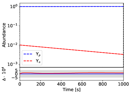
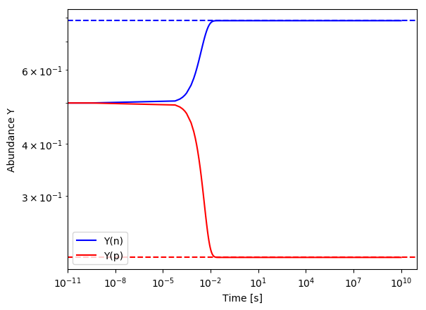
A simple physical test case is the decay of a neutron. This test reveals that mass conservation is not a sufficient convergence criteria if all involved nuclei have the same mass number (i.e., decays). As a consequence, the implementation of the implicit Euler shows large deviations for this simple problem. We compare both, the results of Gears integration method which are close to the analytic solution and the results of the implicit Euler integration method with the ones of a previous version of WinNet. We choose \(Y_n(0)=0.01\) and \(Y_p(0)=0.99\). The decay can be described by the analytical formula:
\[\begin{align} Y_n(t) &= Y_n(0) \cdot e^{-\lambda _n \cdot t} \\ Y_p(t) &= 1- Y_n(t), \end{align}\]
where \(\lambda _n\) is the decay constant of neutrons. The analytical solution is compared to the numerical solution, calculated with WinNet. The sensitivity of the test is set to a relative deviation $\Delta \le 5 \cdot 10^{-4}$ at any time of the calculation.
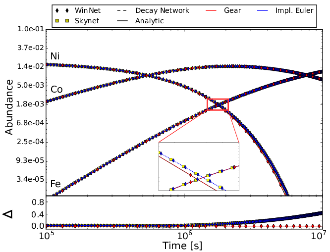
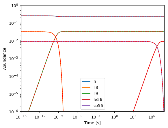
The decay of \(^{56}\)Ni is more complex than the decay of a neutron, since \(^{56}\)Co is included as intermediate decay product. Furthermore, the absence of neutrons and protons in this calculation introduces another test as many routines rely on them (e.g., within WinNet it is not possible to calculate NSE composition without neutrons and protons). This test ensures that neutrons and protons are not explicitly used in parts of the code where it is not necessary. The initial composition is chosen to consist of \(^{56}\)Ni only. The solution to this problem can be calculated analytically:
\[\begin{align} Y_\mathrm{Ni}(t) &= Y_\mathrm{Ni}(0) \cdot e^{- \lambda _{\mathrm{Ni}} \cdot t} \\ Y_\mathrm{Co}(t) &= Y_\mathrm{Co}(0) \cdot e^{- \lambda _{\mathrm{Co}} \cdot t} + Y_\mathrm{Ni}(0) \cdot \frac{\lambda _{\mathrm{Ni}}}{\lambda _{\mathrm{Co}} - \lambda _{\mathrm{Ni}}} \cdot \left( e^{-\lambda _{\mathrm{Ni}}\cdot t} - e^{-\lambda _{\mathrm{Co}}\cdot t} \right)\\ Y_\mathrm{Fe}(t) &= Y_\mathrm{Ni}(0)+Y_\mathrm{Co}(0) - Y_\mathrm{Ni}(t) - Y_\mathrm{Co}(t), \end{align}\]
where \(Y_\mathrm{Ni}\), \(Y_\mathrm{Co}\), and \(Y_\mathrm{Fe}\) are the abundances of \(^{56}\)Ni, \(^{56}\)Co, and \(^{56}\)Fe, respectively, and \(\lambda\) the corresponding decay constants. Similar to the decay of a neutron, the deviation within the implicit Euler method is larger. To test if this is a specific weakness of WinNet, we performed this test in two additional nuclear reaction networks. The figure below shows the time evolution of abundances for the decay of nickel, using different nuclear reaction networks and different integration methods. SkyNet, a python decay network (blue line) and WinNet (blue diamonds) use the implicit Euler method. All codes are in nearly perfect agreement. Using Gears integration method within WinNet (red diamonds) and the python decay network (red dashed line) shows a better agreement with the analytic solution (black line).
In a hot r-process scenario, the reaction path and the \(\beta\)-decay timescales for each isotopic chain are determined by ( \(n,\gamma\))-( \(\gamma,n\)) equilibrium. For this scenario, forward and inverse reactions are involved. The implementation of the inverse reactions in WinNet involves the evaluation of the partition functions. A failure of this test may indicate problems with the implementation of the partition functions. We choose a constant temperature of \(T = 8 \; \mathrm{GK}\) and a density of \(\rho = 10^9 \; \mathrm{g \, cm ^{-3}}\). We include three nuclei, \(^{64}\)Ni, \(^{65}\)Ni, and neutrons and start with an initial composition consisting of \(^{65}\)Ni only. The analytic solution of the involved nuclear reaction network
\[\begin{align} 1 &= Y_\mathrm{n} + 64\cdot Y_\mathrm{^{64}Ni} + 65\cdot Y_\mathrm{^{65}Ni} \\ \frac{28}{65} &= 28\cdot Y_\mathrm{^{64}Ni} + 28\cdot Y_\mathrm{^{65}Ni} \\ 0 &= \dot{Y}_\mathrm{n} = \lambda _{\mathrm{dis}} \cdot Y_\mathrm{^{65}Ni} - \rho \cdot \mathrm{N}_\mathrm{A} \cdot \sigma _\mathrm{capture} \cdot Y_\mathrm{n} Y_\mathrm{^{64}Ni} \end{align} \]
is given by
\[ \begin{align} Y_\mathrm{n} &= \frac{\lambda _{\mathrm{dis}} - \sqrt{\lambda _{\mathrm{dis}}^2 + 4\cdot \rho \, N_\mathrm{A} \, \sigma _{\mathrm{capture}} \, \lambda _{\mathrm{dis}} \cdot 1/65 } }{-2 \cdot \rho \, N_\mathrm{A} \, \sigma _{\mathrm{capture}}} \\ Y_\mathrm{^{64}Ni} &= Y_\mathrm{n} \\ Y_\mathrm{^{65}Ni} &= 1/65 - Y_\mathrm{n}, \end{align} \]
where \(\sigma _{\mathrm{capture}}\) is the reaction rate of \(^{64}\mathrm{Ni}( n,\gamma )^{65}\mathrm{Ni}\) and \(\lambda _{\mathrm{dis}}\) is its inverse reaction rate. This test is performed using Gears integration method, which shows a good agreement with the analytic solution.
| Isotope | \(Y_i\) WinNet | \(Y_i\) analytic | \(\Delta\) |
|---|---|---|---|
| n | \(7.35175\cdot 10^{-3}\) | \(7.35175\cdot 10^{-3}\) | \(1.79\cdot 10^{-9}\) |
| \(^{64}\)Ni | \(7.35175\cdot 10^{-3}\) | \(7.35175\cdot 10^{-3}\) | \(3.17\cdot 10^{-9}\) |
| \(^{65}\)Ni | \(8.03286\cdot 10^{-3}\) | \(8.03286\cdot 10^{-3}\) | \(4.96\cdot 10^{-9}\) |
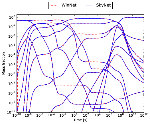
Even with a relatively small number of nuclei, the solution of the nuclear network equations cannot be calculated analytically anymore. Therefore, we test the burning of carbon and oxygen with \(Y_{^{12}\mathrm{C}}(0)=1/24\) and \(Y_{^{16}\mathrm{O}}(0)=1/32\) under hydrostatic conditions. We choose a temperature of \(T=3\,\mathrm{GK}\) and a density of \(\rho = 10^{9}\, \mathrm{g/cm^3}\). The calculation involves \(13\) \(\alpha\)-nuclei from \(^4\)He up to \(^{56}\)Ni. The burning is calculated for \(t=10^{12}\, \mathrm{s}\). We compare the final abundances with SkyNet, where this test is adapted from. The final abundances show a nearly perfect match ( \(\Delta = 8.06\cdot 10^{-4}\)) between WinNet and SkyNet (Figure below) using Gears method.
The synthesis of elements during the first minutes after the creation of our universe can be calculated with a relatively small network. Following Winteler 2013, we create a trajectory for a flat, isotropic, and homogeneous universe to describe the big bang. Furthermore, we assume a freeze-out of weak reactions at \(T=0.8\, \mathrm{MeV}\) and a photon to baryon ratio of \(\eta = 6.11\cdot 10^{-10}\) as measured by the Wilkinson Microwave Anisotropy Prope (WMAP) satellite.
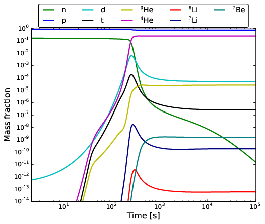
Due to the fast expansion, only light nuclei are synthesized and a small nuclear reaction network is sufficient to describe the problem. We compare the final abundances of this calculation with the final abundances of a reference calculation that has been proven to give reliable results.
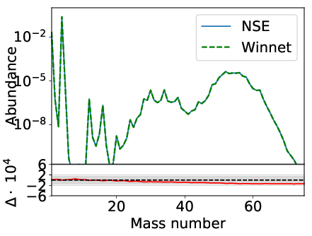
Within this test, we compare the composition of NSE with an external NSE solver. We choose a temperature of \(T=7 \; \mathrm{GK}\), a density of \(\rho = 10^7\, \mathrm{g\,cm^{-3}}\) and an electron fraction of \(Y_e = 0.5\). Furthermore, we do not include screening corrections. This test passes within an accuracy of \(\Delta = 2\cdot 10^{-4}\).
We test the implementation of neutrino reactions by assuming constant electron-neutrino luminosities \(L_e=10^{52}\, \mathrm{erg \,s^{-1}}\), \(\bar{L_e}=5 \cdot 10^{52}\, \mathrm{erg \,s^{-1}}\) and electron-neutrino temperatures \(T_e=8 \, \mathrm{MeV}\), \(\bar{T_e}=10 \, \mathrm{MeV}\). We only include neutrons and protons in this test. After a sufficient time an equilibrium value is obtained, which can be calculated by
\[\begin{align} Y_p &= \left(1+\frac{\bar{L_e}\cdot E_{e}\cdot \bar{\lambda_e} (8\;\mathrm{MeV})}{L_e\cdot \bar{E_{e}} \cdot \lambda_e (10\;\mathrm{MeV})} \right) ^{-1} &=& \, 2.1405\cdot 10^{-2}\\ Y_n &= 1-Y_p &=& \, 7.8595 \cdot 10^{-2}, \end{align}\]
where
\[\begin{equation} E_e = 3.1514 \cdot T_e. \end{equation}\]
This test shows a high accuracy of \(\Delta = 10^{-11}\).
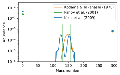
This test performs the \(\beta\)-delayed fission of \(^{295}\mathrm{Am}\). The initial composition consists of \(^{295}\mathrm{Am}\) only and the calculation is done for \(t=10^{-2}\, \mathrm{s}\). We compare the final abundances with the fragment distribution of ABLA (Kelic et al. 2009), Kodama & Takahashi 1976, and Panov et al. 2001.
The nuclear reaction rates in WinNet are implemented using the reaction rate database JINA Reaclib. The format of this database restricts the reaction to a maximum number of four products. However, the \(\beta\)-decay of very neutron rich nuclei involves the release of many neutrons (e.g., up to \(10\) neutrons in the calculation of Moeller et al. 2019). We therefore introduced another format to implement \(\beta\)-decays where all reactions that are also given in the Reaclib file format are replaced. The test calculates the decay of \(^{73}\mathrm{Ca}\) given in \(\beta\)-decay format along with the decay of \(^{24}\mathrm{O}\) given in Reaclib file format.
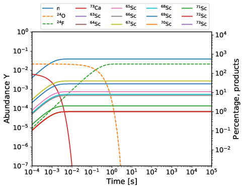
The final abundances can be calculated analytically for the decay of \(^{24}\mathrm{O}\), and result from the probability to emit a neutron in the case of \(^{73}\mathrm{Ca}\). The percentage of each decay product of \(^{73}\mathrm{Ca}\) is in excellent agreement with the input probability for each corresponding decay-channel and the test is set to a sensitivity of \(\Delta < 10^{-5}\).
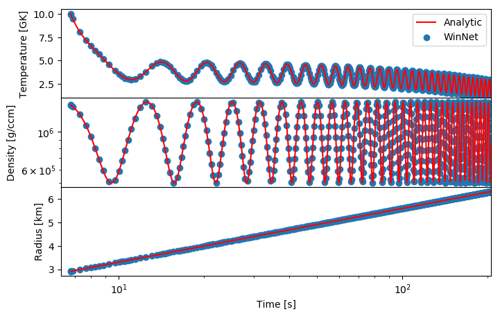
The hydrodynamic conditions can be given by either a trajectory file or an analytic expression. We test that WinNet follows the correct expressions by assuming
\[ \begin{align} T_9 &= \sin(x)+10^{-5} \cdot e^{-x+20}+4-10^{-2} \cdot x \\ \rho &= (5\cdot 10^{-1} \cdot \cos(x)+1) \cdot 10^{6}+\sin(\pi) \\ R &= \ln(x)+1 \end{align} \]
The output is checked with the analytic expression.
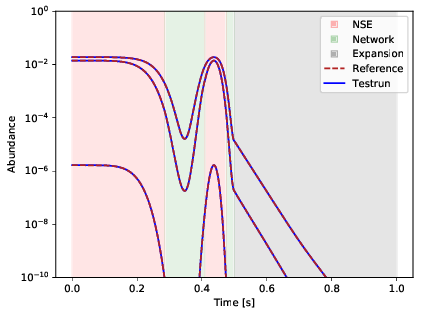
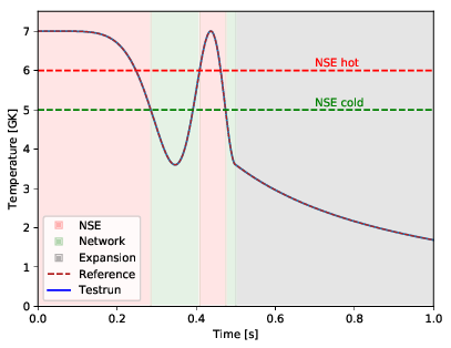
This test ensures that the switches between NSE, Network, and expansion work properly. For this a simple 154 isotope network is calculated with an artificial trajectory. The trajectory was created that it switches between NSE and network several times and that it is short enough that there is an expansion in the end of the simulation. The test passes for \(\Delta < 10^{-3}\).
To ensure that the tabulated rates work as intended, we run a decay in reaclib format together with an \((n, \gamma)\) reaction. The latter reaction is included in the reaclib file as well, but with invalid parameters. The result is compared with a result of a calculation with the same reactions, but all given in reaclib format. The test passes if none of the abundances deviate by more than \(\Delta < 5\cdot 10^{-4}\).
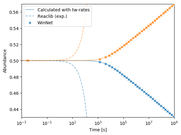
To ensure that the theoretical \(\beta\)-decays and electron captures are working, we run a neutron decay test, but this time with theoretical weak rates enables (iwformat=2). The result is compared with the analytic solution. The test passes if neutrons and protons stay within a deviation of \( \Delta = 5\cdot 10^{-4} \).
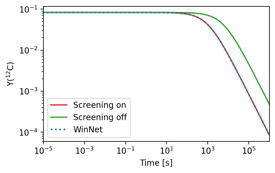
Screening corrections have been tested with the heavy ion \(^{12}\mathrm{C}\) + \(^{12}\mathrm{C}\) reaction. We apply hydrostatic conditions of \( 10^{8}\) g/ccm and 1 GK, evolving pure \(^{12}\mathrm{C}\) matter for \( 10^{6}\) s. The result is compared with an external calculation of the result that has been coded in Python.
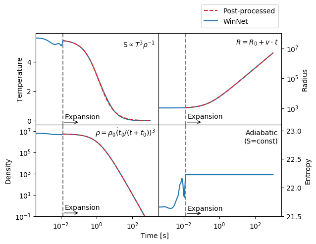
Within this test we ensure that the radius, density, and temperature evolves in a reasonable way during the expansion. In the adiabatic expansion the temperature evolves proportional to
\[ S \propto T^{3}\rho^{-1} \]
Within the test we compare the temperature, density, and radius evolution with a reference run. All quantities have to stay within a deviation of \( \Delta = 10^{-8} \).